XAI¶

The module of xai contains methods that help explain a model decisions.

In order for this module to work properly, Graphiz must be installed. In linux based operating systems use:

sudo apt-get install graphviz

Or using conda:

conda install graphviz

For more information see here.

Draw Tree¶

Deprecated since version 1.6.4: Use sklearn.tree.plot_tree instead

xai.draw_tree(tree: sklearn.tree._classes.BaseDecisionTree, feature_names: Optional[List[str]] = None, class_names: Optional[List[str]] = None, *, ax: Optional[matplotlib.axes._axes.Axes] = None, **kwargs) → matplotlib.axes._axes.Axes[source]¶

Receives a decision tree and return a plot graph of the tree for easy interpretation.

Parameters:	tree – decision tree. feature_names – the features names. class_names – the classes names or labels. ax – Axes object to draw the plot onto, otherwise uses the current Axes. kwargs – other keyword arguments All other keyword arguments are passed to `matplotlib.axes.Axes.pcolormesh()`.
Returns:	Returns the Axes object with the plot drawn onto it.

Code Example¶

In following examples we are going to use the iris dataset from scikit-learn. so firstly let’s import it:

from sklearn import datasets


iris = datasets.load_iris()
x = iris.data
y = iris.target

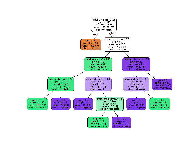
We’ll create a simple decision tree classifier and plot it:

from matplotlib import pyplot
from sklearn.tree import DecisionTreeClassifier

from ds_utils.xai import draw_tree


# Create decision tree classifier object
clf = DecisionTreeClassifier(random_state=0)

# Train model
clf.fit(x, y)

draw_tree(clf, iris.feature_names, iris.target_names)
pyplot.show()

And the following image will be shown:

Draw Dot Data¶

xai.draw_dot_data(dot_data: str, *, ax: Optional[matplotlib.axes._axes.Axes] = None, **kwargs) → matplotlib.axes._axes.Axes[source]¶

Receives a Graphiz’s Dot language string and return a plot graph of the data.

Parameters:	dot_data – Graphiz’s Dot language string. ax – Axes object to draw the plot onto, otherwise uses the current Axes. kwargs – other keyword arguments All other keyword arguments are passed to `matplotlib.axes.Axes.pcolormesh()`.
Returns:	Returns the Axes object with the plot drawn onto it.

Code Example¶

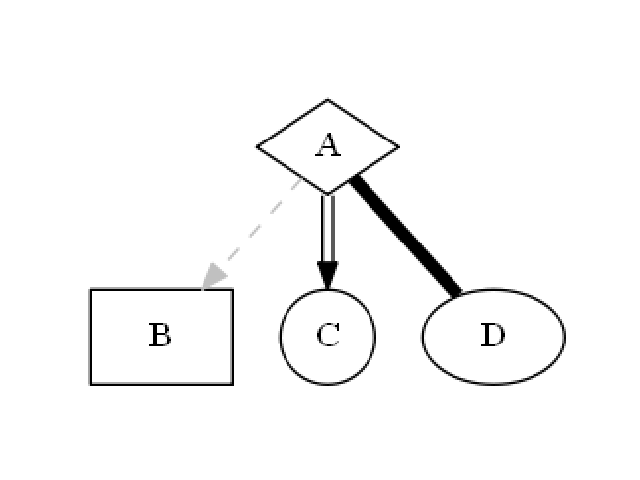
We’ll create a simple diagram and plot it:

from matplotlib import pyplot

from ds_utils.xai import draw_dot_data


dot_data = "digraph D{\n" \
           "\tA [shape=diamond]\n" \
           "\tB [shape=box]\n" \
           "\tC [shape=circle]\n" \
           "\n" \
           "\tA -> B [style=dashed, color=grey]\n" \
           "\tA -> C [color=\"black:invis:black\"]\n" \
           "\tA -> D [penwidth=5, arrowhead=none]\n" \
           "\n" \
           "}"

draw_dot_data(dot_data)
pyplot.show()

And the following image will be shown:

Generate Decision Paths¶

xai.generate_decision_paths(classifier: sklearn.tree._classes.BaseDecisionTree, feature_names: Optional[List[str]] = None, class_names: Optional[List[str]] = None, tree_name: Optional[str] = None, indent_char: str = '\t') → str[source]¶

Receives a decision tree and return the underlying decision-rules (or ‘decision paths’) as text (valid python syntax). Original code

Parameters:	classifier – decision tree. feature_names – the features names. class_names – the classes names or labels. tree_name – the name of the tree (function signature). indent_char – the character used for indentation.
Returns:	textual representation of the decision paths of the tree.

Code Example¶

We’ll create a simple decision tree classifier and print it:

from sklearn.tree import DecisionTreeClassifier

from ds_utils.xai import generate_decision_paths


# Create decision tree classifier object
clf = DecisionTreeClassifier(random_state=0, max_depth=3)

# Train model
clf.fit(x, y)
print(generate_decision_paths(clf, iris.feature_names, iris.target_names.tolist(),
                     "iris_tree"))

The following text will be printed:

def iris_tree(petal width (cm), petal length (cm)):
    if petal width (cm) <= 0.8000:
        # return class setosa with probability 0.9804
        return ("setosa", 0.9804)
    else:  # if petal width (cm) > 0.8000
        if petal width (cm) <= 1.7500:
            if petal length (cm) <= 4.9500:
                # return class versicolor with probability 0.9792
                return ("versicolor", 0.9792)
            else:  # if petal length (cm) > 4.9500
                # return class virginica with probability 0.6667
                return ("virginica", 0.6667)
        else:  # if petal width (cm) > 1.7500
            if petal length (cm) <= 4.8500:
                # return class virginica with probability 0.6667
                return ("virginica", 0.6667)
            else:  # if petal length (cm) > 4.8500
                # return class virginica with probability 0.9773
                return ("virginica", 0.9773)

Plot Features` Importance¶

xai.plot_features_importance(feature_names: List[str], feature_importance: List[float], *, ax: Optional[matplotlib.axes._axes.Axes] = None, **kwargs) → matplotlib.axes._axes.Axes[source]¶

plot feature importance as a bar chart.

Parameters:	feature_names – strings list of feature names feature_importance – float list of feature importance ax – Axes object to draw the plot onto, otherwise uses the current Axes. kwargs – other keyword arguments All other keyword arguments are passed to `matplotlib.axes.Axes.pcolormesh()`.
Returns:	Returns the Axes object with the plot drawn onto it.

Code Example¶

For this example I created a dummy data set. You can find the data at the resources directory in the packages tests folder.

Let’s see how to use the code:

import pandas

from matplotlib import pyplot
from sklearn.preprocessing import OneHotEncoder
from sklearn.tree import DecisionTreeClassifier

from ds_utils.xai import plot_features_importance


data_1M = pandas.read_csv(path/to/dataset)
target = data_1M["x12"]
categorical_features = ["x7", "x10"]
for i in range(0, len(categorical_features)):
    enc = OneHotEncoder(sparse=False, handle_unknown="ignore")
    enc_out = enc.fit_transform(data_1M[[categorical_features[i]]])
    for j in range(0, len(enc.categories_[0])):
        data_1M[categorical_features[i] + "_" + enc.categories_[0][j]] = enc_out[:, j]
features = data_1M.columns.to_list()
features.remove("x12")
features.remove("x7")
features.remove("x10")

clf = DecisionTreeClassifier(random_state=42)
clf.fit(data_1M[features], target)
plot_features_importance(features, clf.feature_importances_)

pyplot.show()

And the following image will be shown: