Receiver Operating Characteristic (ROC) Curve with Probabilities (Thresholds) Annotations

The ROC curve is a graphical plot that illustrates the diagnostic ability of a binary classifier system as its discrimination threshold is varied. It plots the True Positive Rate (TPR) against the False Positive Rate (FPR) at various threshold settings. The ROC curve is particularly useful when you have balanced classes or when you want to evaluate the classifier’s performance across all possible thresholds.

ds_utils.metrics.curves.plot_roc_curve_with_thresholds_annotations(y_true: ndarray, classifiers_names_and_scores_dict: Dict[str, ndarray], *, positive_label: int | float | bool | str | None = None, sample_weight: ndarray | None = None, drop_intermediate: bool = True, average: str | None = 'macro', max_fpr: float | None = None, multi_class: str = 'raise', labels: ndarray | None = None, fig: Figure | None = None, mode: str | None = 'lines+markers', add_random_classifier_line: bool = True, random_classifier_line_kw: Dict | None = None, show_legend: bool = True, **kwargs) → Figure[source]

Plot ROC curves with threshold annotations for multiple classifiers.

Parameters:

y_true – array-like of shape (n_samples,). True binary labels.
classifiers_names_and_scores_dict – mapping from classifier name to classifier’s score.
positive_label – int, float, bool or str, default=None. The label of the positive class.
sample_weight – array-like of shape (n_samples,), default=None. Sample weights.
drop_intermediate – bool, default=True. Whether to drop some suboptimal thresholds which would not appear on a plotted ROC curve.
average – {‘micro’, ‘macro’, ‘samples’, ‘weighted’} or None, default=’macro’. If not None, this determines the type of averaging performed on the data.
max_fpr – float > 0 and <= 1, default=None. If not None, the standardized partial AUC over the range [0, max_fpr] is returned.
multi_class – {‘raise’, ‘ovr’, ‘ovo’}, default=’raise’. Determines the type of configuration to use for multiclass targets.
labels – array-like of shape (n_classes,), default=None. Only used for multiclass targets. List of labels that index the classes in y_score.
fig – plotly’s Figure object, optional. The figure to plot on.
mode – str, default=’lines+markers’. Determines the drawing mode for this scatter trace.
add_random_classifier_line – bool, default=True. Whether to plot a diagonal dashed black line which represents a random classifier.
random_classifier_line_kw – dict, default=None. Keyword arguments to be passed to plotly’s Scatter for rendering the random classifier line (e.g., line color, style).
show_legend – bool, default=True. Whether to display legend in the plot.
kwargs – additional keyword arguments to be passed to the plot function.

Returns:

The Figure object with the plot drawn onto it.

Raises:

ValueError – If the input data is invalid or inconsistent.

Code Example

Suppose that we want to compare 3 classifiers based on ROC Curve and optimize the prediction threshold. The method uses Plotly as the backend engine to create the graphs and adds the AUC score next to each classifier name:

from sklearn.tree import DecisionTreeClassifier
from sklearn.ensemble import RandomForestClassifier
from xgboost import XGBClassifier

from ds_utils.metrics.curves import plot_roc_curve_with_thresholds_annotations

# Define and train classifiers
tree_clf = DecisionTreeClassifier(random_state=42)
rf_clf = RandomForestClassifier(random_state=42)
xgb_clf = XGBClassifier(random_state=42, eval_metric='logloss')

tree_clf.fit(X_train, y_train)
rf_clf.fit(X_train, y_train)
xgb_clf.fit(X_train, y_train)

# Prepare classifier predictions
classifiers_names_and_scores_dict = {
    "Decision Tree": tree_clf.predict_proba(X_test)[:, 1],
    "Random Forest": rf_clf.predict_proba(X_test)[:, 1],
    "XGBoost": xgb_clf.predict_proba(X_test)[:, 1]
}

# Plot ROC curves
fig = plot_roc_curve_with_thresholds_annotations(
    y_test,
    classifiers_names_and_scores_dict,
    positive_label=1
)
fig.show()

The positive_label=1 parameter specifies which class should be considered as the positive class when calculating the ROC curve. In this case, it indicates that the class labeled as ‘1’ is the positive class.

And the following interactive graph will be shown:

Receiver Operating Characteristic (ROC) Curve with Probabilities (Thresholds) Annotations

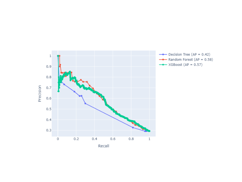
Precision-Recall Curve with Probabilities (Thresholds) Annotations

The Precision-Recall curve shows the tradeoff between precision and recall for different threshold values. It is particularly useful when you have imbalanced classes, as it focuses on the performance of the positive class. Precision-Recall curves are preferred over ROC curves when you have a large skew in the class distribution, as they are more sensitive to differences in the minority class.

ds_utils.metrics.curves.plot_precision_recall_curve_with_thresholds_annotations(y_true: ndarray, classifiers_names_and_scores_dict: Dict[str, ndarray], *, positive_label: int | float | bool | str | None = None, sample_weight: ndarray | None = None, drop_intermediate: bool = True, fig: Figure | None = None, mode: str | None = 'lines+markers', plot_chance_level: bool = False, chance_level_kw: Dict | None = None, show_legend: bool = True, **kwargs) → Figure[source]

Plot Precision-Recall curves with threshold annotations for multiple classifiers.